import fingertips_py as ftp

import pandas as pdWalkthrough of fingertips_py
In conjunction with the tutorial on webscraping and APIs, below is a walkthrough of the fingertips_py package maintained by the Department of Health and Social Care, which simplifies importing data via the Fingertips API.
Documentation
Fingertips Public Health Profiles (public-facing source of the data)
Installation
For more information, see the fingertips_py documentation.
Code Club recommends using the uv package management software, but if you do need to use pip, the relevant installation instructions are below.
uv
To install using uv, enter the following in the terminal:
uv add fingertips_pypip
To install using pip, activate your environment and enter the following in the terminal:
python -m pip install fingertips_pyExploring package functionality
Let’s have a look at the various methods in the package that allow us to import different levels of the dataset and the metadata.
Importing the package
We will also use pandas for presenting the imported data in a dataframe.
Get profile IDs by profile name
The profile IDs can be used to refer to different “profiles” on Fingertips. That is to say, different aspects of public health such as levels of diabetes, cardiovascular disease, or dementia in the country.
# Cancer profile ID
cancer_profile_md = ftp.metadata.get_profile_by_name('cancer services') # creates a dictionary of metadata. Profile names are not case sensitive.

cancer_profile_id = cancer_profile_md['Id'] # access the profile ID in the metadata dictionary

# Wider Determinants of Health profile ID

wdoh_profile_md = ftp.metadata.get_profile_by_name('wider determinants of health')

wdoh_profile_id = wdoh_profile_md['Id']

# Return the IDs

print(f'Cancer profile ID: {cancer_profile_id}')
print(f'Wider Determinants of Health profile ID: {wdoh_profile_id}')
Cancer profile ID: 92
Wider Determinants of Health profile ID: 130Get profile metadata as a dataframe
Inspecting the metadata gives you a lot of information about a given profile, such as metric sources, definition, and polarity.
wdoh_md_df = ftp.metadata.get_metadata_for_profile_as_dataframe(wdoh_profile_id)

wdoh_md_df.head()| Indicator ID | Indicator | Indicator number | Rationale | Specific rationale | Definition | Data source | Indicator source | Definition of numerator | Source of numerator | ... | Data re-use | Links | Indicator Content | Simple Name | Simple Definition | Unit | Value type | Year type | Polarity | Date updated | |
|---|---|---|---|---|---|---|---|---|---|---|---|---|---|---|---|---|---|---|---|---|---|
| 0 | 11401 | The rate of complaints about noise | B14a | The Government's policy on noise is set out in... | NaN | Number of complaints per year per local author... | OHID, in collaboration with Chartered Institut... | Data on noise complaints provided by Chartered... | Number of complaints about noise. | Chartered Institute of Environmental Health (C... | ... | NaN | http://www.cieh.org/ | NaN | NaN | NaN | per 1,000 | Crude rate | Financial | RAG - Low is good | 11/04/2025 |
| 1 | 93754 | Killed and seriously injured casualties on Eng... | B10 | Motor vehicle traffic accidents are a major ca... | NaN | Number of people reported killed or seriously ... | OHID, based on Department for Transport data | NaN | The number of people of all ages killed or ser... | Department for Transport (DfT), Road accidents... | ... | Killed and seriously injured data are National... | <span style="color: #0b0c0c; font-family: GDS ... | NaN | People killed or seriously injured on roads | Rate of people reported killed or seriously in... | per billion vehicle miles | Crude rate | Calendar | RAG - Low is good | 22/10/2025 |
| 2 | 93074 | Access to Healthy Assets & Hazards Index | NaN | The Access to Healthy Assets and Hazards (AHAH... | NaN | Percentage of the population who live in LSOAs... | Consumer Data Research Centre | The overall index collates data from a variety... | Total population residing in Lower Super Outpu... | Consumer Data Research Centre (CDRC), Access t... | ... | NaN | https://data.cdrc.ac.uk/dataset/access-healthy... | NaN | NaN | NaN | % | Proportion | Calendar | RAG - Low is good | 03/09/2024 |
| 3 | 90357 | The percentage of the population exposed to ro... | B14b | There are a number of direct and indirect link... | NaN | Noise exposure determined by strategic noise m... | OHID, based on Department for Environment, Foo... | NaN | Noise exposure determined by strategic noise m... | Department for Environment, Food and Rural Aff... | ... | NaN | NaN | NaN | NaN | NaN | % | Proportion | Calendar | RAG - Low is good | 23/01/2025 |
| 4 | 94124 | Fast food outlets per 100,000 population | NaN | <p class="MsoNormal" style="margin-bottom: 0cm... | NaN | <p class="MsoNormal" style="margin-bottom: 0cm... | OHID, based on Food Standards Agency data | NaN | <span style="line-height: 107%; mso-fareast-fo... | Food Standards Agency (FSA), Food Hygiene Rati... | ... | NaN | NaN | NaN | NaN | NaN | per 100,000 | Crude rate | Calendar | RAG - Low is good | 24/01/2025 |
5 rows × 32 columns
Get metadata by indicator ID
fast_food_md = ftp.get_metadata_for_indicator_as_dataframe(94124)

fast_food_md| Indicator ID | Indicator | Indicator number | Rationale | Specific rationale | Definition | Data source | Indicator source | Definition of numerator | Source of numerator | ... | Data re-use | Links | Indicator Content | Simple Name | Simple Definition | Unit | Value type | Year type | Polarity | Date updated | |
|---|---|---|---|---|---|---|---|---|---|---|---|---|---|---|---|---|---|---|---|---|---|
| 0 | 94124 | Fast food outlets per 100,000 population | NaN | <p class="MsoNormal" style="margin-bottom: 0cm... | NaN | <p class="MsoNormal" style="margin-bottom: 0cm... | OHID, based on Food Standards Agency data | NaN | <span style="line-height: 107%; mso-fareast-fo... | Food Standards Agency (FSA), Food Hygiene Rati... | ... | NaN | NaN | NaN | NaN | NaN | per 100,000 | Crude rate | Calendar | RAG - Low is good | 24/01/2025 |
1 rows × 32 columns
Get all area types
This can help you understand which geographical breakdowns are available via the API. The code below just returns the first 10 so that a large table doesn’t get displayed on this page, but there are many more. Worth looking into, if you are planning to make use of these metrics to support the narrative in a report you are working on.
# returns a nested dictionary, where the area ID is the key to a further dictionary of key:value pairs
all_areas_dict = ftp.metadata.get_all_areas()

# converts the nested dictionary to a DataFrame, where the outer key becomes the index
all_areas_df = pd.DataFrame.from_dict(all_areas_dict, orient='index')

# reset the DataFrame to have the default indexing
all_areas_df = all_areas_df.reset_index()

# rename the column labelled 'index' in the dictionary-to-DataFrame conversion
all_areas_df.rename(columns={'index':'Id'}, inplace=True)

all_areas_df.head(10)| Id | Name | Short | Class | Sequence | CanBeDisplayedOnMap | |
|---|---|---|---|---|---|---|
| 0 | 3 | Middle Super Output Area | MSOA | None | 0 | True |
| 1 | 6 | Government Office Region (E12) | Regions (statistical) | None | 0 | True |
| 2 | 7 | General Practice | GPs | gp | 0 | True |
| 3 | 8 | Electoral Best Fit Wards (2024) | Electoral Wards (2024) | None | 0 | True |
| 4 | 9 | Census Merged Wards | Merged Wards | None | 0 | False |
| 5 | 14 | Acute Trust | Acute Trust | None | 0 | False |
| 6 | 15 | England | England | None | 0 | False |
| 7 | 20 | Mental Health Trust | Mental Health Trust | None | 0 | False |
| 8 | 41 | Ambulance Trust | Ambulance Trust | None | 0 | False |
| 9 | 66 | Sub-ICB, former CCGs | ICB sub-locations | None | 2022 | True |
Get all area types available for a particular profile
wdoh_areas = ftp.metadata.get_area_types_for_profile(wdoh_profile_id)

wdoh_areas_df = pd.DataFrame.from_dict(wdoh_areas, orient='index')

wdoh_areas_df.reset_index(inplace=True)

wdoh_areas_df.drop('index', axis=1,inplace=True) # drop the column called 'index' following the dictionary-to-DataFrame conversion

wdoh_areas_df| Name | Short | Class | CanBeDisplayedOnMap | Sequence | Id | |
|---|---|---|---|---|---|---|
| 0 | Government Office Region (E12) | Regions (statistical) | None | True | 0 | 6 |
| 1 | England | England | None | False | 0 | 15 |
| 2 | Lower tier local authorities (post 4/23) | Districts & UAs (from Apr 2023) | ua-la-composite | True | 2023 | 501 |
| 3 | Upper tier local authorities (post 4/23) | Counties & UAs (from Apr 2023) | ua-county-composite | True | 2023 | 502 |
Get all data for indicators
There seems to be an error within this function at time of writing since it constructs an invalid URL. It has been kept in this demonstration so that you can be made aware that this method may not work, unless it has been fixed.
ftp.retrieve_data.get_all_data_for_indicators
wdoh_indicators_df = pd.DataFrame(
    ftp.retrieve_data.get_all_data_for_indicators(
        [11404,92772],                  # two Wider Determinants of Health indicators
         502,                           # Area type = Upper tier local authorities
         15,                            # Parent area type =  England
         filter_by_area_codes= None,
         is_test= False
    )
)

wdoh_indicators_df.head()
Let’s try this one instead
This one does much the same thing, though slightly differently, while not causing an error.
fingertips_py.retrieve_data.get_data_by_indicator_ids
wdoh_indicators_df = pd.DataFrame(
    ftp.retrieve_data.get_data_by_indicator_ids(
        [11404,92772],                          # two Wider Determinants of Health indicators
         502,                                   # Area type = Upper tier local authorities
         15,                                    # Parent area type =  England
         include_sortable_time_periods=None,
         is_test= False
    )
)

wdoh_indicators_df.head()| Indicator ID | Indicator Name | Parent Code | Parent Name | Area Code | Area Name | Area Type | Sex | Age | Category Type | ... | Count | Denominator | Value note | Recent Trend | Compared to England value or percentiles | Compared to percentiles | Time period Sortable | New data | Compared to goal | Time period range | |
|---|---|---|---|---|---|---|---|---|---|---|---|---|---|---|---|---|---|---|---|---|---|
| 0 | 92772 | Premises licensed to sell alcohol per square k... | NaN | NaN | E92000001 | England | England | Not applicable | Not applicable | NaN | ... | 154487.0 | 130310.0136 | Aggregated from all known lower geography values | NaN | Not compared | Not compared | 20150000 | NaN | NaN | 1y |
| 1 | 92772 | Premises licensed to sell alcohol per square k... | E92000001 | England | E92000001 | England | England | Not applicable | Not applicable | NaN | ... | 154487.0 | 130310.0136 | Aggregated from all known lower geography values | NaN | Similar | Not compared | 20150000 | NaN | NaN | 1y |
| 2 | 92772 | Premises licensed to sell alcohol per square k... | E92000001 | England | E06000001 | Hartlepool | Counties & UAs (from Apr 2023) | Not applicable | Not applicable | NaN | ... | 312.0 | 93.5595 | NaN | NaN | Worse | Not compared | 20150000 | NaN | NaN | 1y |
| 3 | 92772 | Premises licensed to sell alcohol per square k... | E92000001 | England | E06000002 | Middlesbrough | Counties & UAs (from Apr 2023) | Not applicable | Not applicable | NaN | ... | 347.0 | 53.8888 | NaN | NaN | Worse | Not compared | 20150000 | NaN | NaN | 1y |
| 4 | 92772 | Premises licensed to sell alcohol per square k... | E92000001 | England | E06000003 | Redcar and Cleveland | Counties & UAs (from Apr 2023) | Not applicable | Not applicable | NaN | ... | 361.0 | 244.8202 | NaN | NaN | Worse | Not compared | 20150000 | NaN | NaN | 1y |
5 rows × 27 columns
Get data at all available geographies for a particular indicator
licensed_premises_all_geographies = ftp.retrieve_data.get_data_for_indicator_at_all_available_geographies(92772)

licensed_premises_all_geographies.head()| Indicator ID | Indicator Name | Parent Code | Parent Name | Area Code | Area Name | Area Type | Sex | Age | Category Type | ... | Count | Denominator | Value note | Recent Trend | Compared to England value or percentiles | Compared to percentiles | Time period Sortable | New data | Compared to goal | Time period range | |
|---|---|---|---|---|---|---|---|---|---|---|---|---|---|---|---|---|---|---|---|---|---|
| 0 | 92772 | Premises licensed to sell alcohol per square k... | NaN | NaN | E92000001 | England | England | Not applicable | Not applicable | NaN | ... | 154487.0 | 130310.0136 | Aggregated from all known lower geography values | NaN | Not compared | Not compared | 20150000 | NaN | NaN | 1y |
| 1 | 92772 | Premises licensed to sell alcohol per square k... | E92000001 | England | E92000001 | England | England | Not applicable | Not applicable | NaN | ... | 154487.0 | 130310.0136 | Aggregated from all known lower geography values | NaN | Similar | Not compared | 20150000 | NaN | NaN | 1y |
| 2 | 92772 | Premises licensed to sell alcohol per square k... | E92000001 | England | E06000001 | Hartlepool | Counties & UAs (from Apr 2023) | Not applicable | Not applicable | NaN | ... | 312.0 | 93.5595 | NaN | NaN | Worse | Not compared | 20150000 | NaN | NaN | 1y |
| 3 | 92772 | Premises licensed to sell alcohol per square k... | E92000001 | England | E06000002 | Middlesbrough | Counties & UAs (from Apr 2023) | Not applicable | Not applicable | NaN | ... | 347.0 | 53.8888 | NaN | NaN | Worse | Not compared | 20150000 | NaN | NaN | 1y |
| 4 | 92772 | Premises licensed to sell alcohol per square k... | E92000001 | England | E06000003 | Redcar and Cleveland | Counties & UAs (from Apr 2023) | Not applicable | Not applicable | NaN | ... | 361.0 | 244.8202 | NaN | NaN | Worse | Not compared | 20150000 | NaN | NaN | 1y |
5 rows × 27 columns
Let’s check whether it has included all geographies by getting a list of unique area types
set(licensed_premises_all_geographies['Area Type']){'Counties & UAs (2021/22-2022/23)',
'Counties & UAs (from Apr 2023)',
'Districts & UAs (2021/22-2022/23)',
'Districts & UAs (from Apr 2023)',
'England',
'Regions (statistical)'}Let’s put all this together and visualise it on a map
We will need to import some more packages:
- Geopandas: supports combining geographical data with
pandasDataFrames. - Contextily: used for laying maps over geographical shapes, such as maps provided by OpenStreetMap.
- Matplotlib: user for applying shading to geographical shapes, adding a legend and any other useful chart elements.
import geopandas as gpd
import matplotlib.pyplot as plt
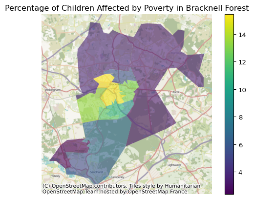
import contextily as cxLet’s plot “Child Poverty, Income deprivation affecting children index (IDACI) 2019 Proportion %” in Bracknell Forest Local Authority area by MSOA. Let’s imagine we found this metric on the Fingertips website and want to import the data so that we can create a custom visualisation to go into some background narrative to a report.
Firstly, we need the profile ID for the Profile “Local health, public health data for small geographic areas”. Then we can get the profile metadata as a dataframe so that we can see how the metric we are interested is referred to within the dataset.
small_geographic_areas_md = ftp.metadata.get_profile_by_name('Local health, public health data for small geographic areas')

# access the profile ID in the metadata dictionary
small_geographic_areas_id = small_geographic_areas_md['Id']

# get a metadata dataframe for the profile in question
small_geographic_areas_md_df = ftp.metadata.get_metadata_for_profile_as_dataframe(small_geographic_areas_id)

# get the indicator ID and name where the name contains "IDACI"
idaci = small_geographic_areas_md_df[['Indicator ID','Indicator']][small_geographic_areas_md_df['Indicator'].str.contains('IDACI')]

# inspect the metrics in our "idaci" variable
idaci| Indicator ID | Indicator | |
|---|---|---|
| 6 | 93094 | Children in poverty: Income Deprivation Affect... |
There’s only one indicator with “IDACI” in the name, so we can go ahead and use the indicator ID to get the data for the metric we are interested in at MSOA level.
idaci_id = idaci['Indicator ID'].iloc[0] # gets the entry from the Indicator ID column

idaci_df = pd.DataFrame(
    ftp.retrieve_data.get_data_by_indicator_ids(
        idaci_id,
        3, # MSOA
        501 # Local Authority
    )
)

idaci_df.head()| Indicator ID | Indicator Name | Parent Code | Parent Name | Area Code | Area Name | Area Type | Sex | Age | Category Type | ... | Count | Denominator | Value note | Recent Trend | Compared to England value or percentiles | Compared to Districts & UAs (from Apr 2023) value or percentiles | Time period Sortable | New data | Compared to goal | Time period range | |
|---|---|---|---|---|---|---|---|---|---|---|---|---|---|---|---|---|---|---|---|---|---|
| 0 | 93094 | Children in poverty: Income Deprivation Affect... | NaN | NaN | E92000001 | England | England | Persons | <16 yrs | NaN | ... | 1777641.757 | 10405050 | NaN | Cannot be calculated | Not compared | Not compared | 20190000 | NaN | NaN | 1y |
| 1 | 93094 | Children in poverty: Income Deprivation Affect... | E92000001 | England | E06000001 | Hartlepool | Districts & UAs (from Apr 2023) | Persons | <16 yrs | NaN | ... | 4978.719 | 17580 | NaN | Cannot be calculated | Worse | Not compared | 20190000 | NaN | NaN | 1y |
| 2 | 93094 | Children in poverty: Income Deprivation Affect... | E92000001 | England | E06000002 | Middlesbrough | Districts & UAs (from Apr 2023) | Persons | <16 yrs | NaN | ... | 9359.504 | 28622 | NaN | Cannot be calculated | Worse | Not compared | 20190000 | NaN | NaN | 1y |
| 3 | 93094 | Children in poverty: Income Deprivation Affect... | E92000001 | England | E06000003 | Redcar and Cleveland | Districts & UAs (from Apr 2023) | Persons | <16 yrs | NaN | ... | 6195.212 | 24210 | NaN | Cannot be calculated | Worse | Not compared | 20190000 | NaN | NaN | 1y |
| 4 | 93094 | Children in poverty: Income Deprivation Affect... | E92000001 | England | E06000004 | Stockton-on-Tees | Districts & UAs (from Apr 2023) | Persons | <16 yrs | NaN | ... | 7965.449 | 38168 | NaN | Cannot be calculated | Worse | Not compared | 20190000 | NaN | NaN | 1y |
5 rows × 27 columns
Now we can import the data for the geographic mapping. For this we will use a .geojson boundary shape file downloaded from the Open Geography Portal.
gdf = gpd.read_file('data/MSOA_Dec_2011_Boundaries_Super_Generalised_Clipped_BSC_EW_V3_2022_-5254045062471510471.geojson')

gdf.head()| OBJECTID | MSOA11CD | MSOA11NM | MSOA11NMW | BNG_E | BNG_N | LONG | LAT | GlobalID | geometry | |
|---|---|---|---|---|---|---|---|---|---|---|
| 0 | 1 | E02000001 | City of London 001 | City of London 001 | 532378 | 181354 | -0.093570 | 51.51560 | a9f03568-7a0a-42b8-a23e-1271f76431e1 | POLYGON ((-0.08519 51.52034, -0.07845 51.52151... |
| 1 | 2 | E02000002 | Barking and Dagenham 001 | Barking and Dagenham 001 | 548267 | 189693 | 0.138759 | 51.58659 | f0ca54f0-1a1e-4c72-8fcb-85e21be6de79 | POLYGON ((0.14984 51.59701, 0.15111 51.58708, ... |
| 2 | 3 | E02000003 | Barking and Dagenham 002 | Barking and Dagenham 002 | 548259 | 188522 | 0.138150 | 51.57607 | 3772a2ec-b052-4000-b62b-2c85ac401a7f | POLYGON ((0.14841 51.58075, 0.14978 51.5697, 0... |
| 3 | 4 | E02000004 | Barking and Dagenham 003 | Barking and Dagenham 003 | 551004 | 186418 | 0.176830 | 51.55644 | 3388e1f6-e578-4907-b271-168756f05856 | POLYGON ((0.19021 51.55268, 0.18602 51.54754, ... |
| 4 | 5 | E02000005 | Barking and Dagenham 004 | Barking and Dagenham 004 | 548733 | 186827 | 0.144269 | 51.56071 | 1af0aed4-60d0-4fd6-b326-4b868968c12f | POLYGON ((0.15441 51.56607, 0.1479 51.56109, 0... |
Next, we join it to the Fingertips data so that the metric data and the geographical data are all in one dataframe.
boundary_df = pd.merge(
    left= gdf,
    right= idaci_df,
    left_on= 'MSOA11CD',
    right_on= 'Area Code',
    how= 'right'
)

boundary_df = boundary_df[boundary_df['Parent Name'] == 'Bracknell Forest'] # just get data where the parent area (i.e. local authority) is Bracknell Forest

boundary_df.head()| OBJECTID | MSOA11CD | MSOA11NM | MSOA11NMW | BNG_E | BNG_N | LONG | LAT | GlobalID | geometry | ... | Count | Denominator | Value note | Recent Trend | Compared to England value or percentiles | Compared to Districts & UAs (from Apr 2023) value or percentiles | Time period Sortable | New data | Compared to goal | Time period range | |
|---|---|---|---|---|---|---|---|---|---|---|---|---|---|---|---|---|---|---|---|---|---|
| 3497 | 3263.0 | E02003352 | Bracknell Forest 001 | Bracknell Forest 001 | 491853.0 | 172163.0 | -0.67980 | 51.44102 | 3c549766-9728-4db5-b739-7c766b7413c1 | POLYGON ((-0.65676 51.46149, -0.65822 51.44932... | ... | 34.968 | 1018 | NaN | Cannot be calculated | Better | Better | 20190000 | NaN | NaN | 1y |
| 3498 | 3264.0 | E02003353 | Bracknell Forest 002 | Bracknell Forest 002 | 486081.0 | 171506.0 | -0.76298 | 51.43602 | ae2b8239-e38a-4f1c-90fe-f290fbc538e8 | POLYGON ((-0.75275 51.46223, -0.74107 51.45887... | ... | 64.414 | 1752 | NaN | Cannot be calculated | Better | Better | 20190000 | NaN | NaN | 1y |
| 3499 | 3265.0 | E02003354 | Bracknell Forest 003 | Bracknell Forest 003 | 487683.0 | 170212.0 | -0.74026 | 51.42414 | 31f3071a-3138-4059-b9cd-279441b78d10 | POLYGON ((-0.72071 51.41979, -0.72078 51.41927... | ... | 117.612 | 2124 | NaN | Cannot be calculated | Better | Better | 20190000 | NaN | NaN | 1y |
| 3500 | 3266.0 | E02003355 | Bracknell Forest 004 | Bracknell Forest 004 | 486030.0 | 169758.0 | -0.76414 | 51.42031 | 74e3802a-22fa-476d-9574-9987b0adabb0 | POLYGON ((-0.75417 51.41869, -0.76013 51.41353... | ... | 234.014 | 1515 | NaN | Cannot be calculated | Similar | Worse | 20190000 | NaN | NaN | 1y |
| 3501 | 3267.0 | E02003356 | Bracknell Forest 005 | Bracknell Forest 005 | 490476.0 | 167562.0 | -0.70078 | 51.39988 | 3905ed89-433e-4322-8e30-e7c16404ebe1 | POLYGON ((-0.68535 51.40142, -0.66763 51.38457... | ... | 46.210 | 1470 | NaN | Cannot be calculated | Better | Better | 20190000 | NaN | NaN | 1y |
5 rows × 37 columns
Finally, we can plot the data onto OpenStreetMap using the contextily package.
matplotlib.pyplot plots the boundary shapes coloured by percentage using the polygon geometry data from the geopandas dataframe.
ax = boundary_df.plot(column= 'Value', legend=True, alpha = 0.6)

ax.axis('off')
ax.set_title('Percentage of Children Affected by Poverty in Bracknell Forest')

cx.add_basemap(
    ax,
    crs=boundary_df.crs.to_string()
)