import numpy as np
import matplotlib.pyplot as plt
import pandas as pd
import seaborn as sns

from sklearn.model_selection import train_test_split
from sklearn.linear_model import LogisticRegression
from sklearn.metrics import accuracy_score, confusion_matrix, ConfusionMatrixDisplay

# set random seed for reproducibility
np.random.seed(42)Introduction to Machine Learning
This is the first session in our machine learning series. This session will focus on introducing machine learning conceptually. We will first discuss what machine learning is and why it is so powerful, then build a simple model to predict passenger survival on the Titanic. The goal is not to come away from this session with a complete, thorough understanding of machine learning. Instead, the goal is to understand what machine learning brings to the table.
Slides
Use the left ⬅️ and right ➡️ arrow keys to navigate through the slides below. To view in a separate tab/window, follow this link.
What is Machine Learning?
In analytics and data science, tasks often focus on explaining why something happened or predicting what will happen in the future. Both of these tasks are complex, but for different reasons. Predicting the future is difficult because data can only tell us about the past. There are a number of ways we can approach this problem, but in the NHS, we often rely on dashboards that describe what has happened in the past to inform decisions about the future. This is inherently limited because many factors will cause the future to differ from the past, and decision-making based on descriptions of the past relies heavily on human judgment.
We can improve on human judgment using rules-based systems, which define explicit rules (IF condition THEN action) to generate predictions1. This can be effective in simple contexts where the rules are already known and easily quantified, but struggle with any complexity. Another approach to making decisions about the future more robust is statistical modelling; however, traditional statistical methods can struggle with large numbers of variables, complex and unknown interactions, and predictions that need to be automated and applied at scale.
This is where machine learning comes in. Machine learning is an approach to building systems that learn patterns from data to make predictions about the future. Fundamentally, machine learning is a blend of statistics and software development, leveraging statistical methods and applying software development principles to solve the problems of complexity and scale. The result is systems that are highly effective at predicting outcomes, can be applied at scale, and deployed in the real world to have a meaningful impact on our decisions about the future.
Machine learning can be applied to a wide variety of contexts and can work with all types of data, structured and unstructured2. In healthcare, there are lots of examples where machine learning can be very effective:
- Readmission Prediction - Which patients need follow-up care?
- Diagnostic Support - Which patients need further testing?
- Resource Allocation - How many beds needed next week?
- Treatment Personalisation - Which intervention works for whom?
Predicting Survival on the Titanic
We will use a classic machine learning dataset, passenger data from the Titanic, to demonstrate what a simple model looks like and how machine learning works. The task is to predict passenger survival. This is a type of task called supervised learning, where you train a model on data where the outcome is already known and labelled, in order to predict answers on new data for which the outcome is not known.
For example, predicting future readmissions from patient data that has an outcome variable that tells us whether patients were readmitted or not is a supervised learning task.
The basic machine learning workflow, which will be demonstrated below, looks as follows:
- Get data with examples and labels
- Split into training and testing sets
- Train a model on training data
- Predict on test data
- Evaluate how well it performed
Setup
First, let’s import the libraries we need, and the titanic dataset.
# load the titanic dataset
df = sns.load_dataset('titanic')
Data Exploration
Before building our model we should explore the data to help us make decisions about how to transform the data so it is ready for modelling and how to structure our model.
In practice, the exploratory phase should be much more detailed, but here we will keep it simple and focus on demonstrating the basic machine learning workflow.
# inspect first few rows
df.head()| survived | pclass | sex | age | sibsp | parch | fare | embarked | class | who | adult_male | deck | embark_town | alive | alone | |
|---|---|---|---|---|---|---|---|---|---|---|---|---|---|---|---|
| 0 | 0 | 3 | male | 22.0 | 1 | 0 | 7.2500 | S | Third | man | True | NaN | Southampton | no | False |
| 1 | 1 | 1 | female | 38.0 | 1 | 0 | 71.2833 | C | First | woman | False | C | Cherbourg | yes | False |
| 2 | 1 | 3 | female | 26.0 | 0 | 0 | 7.9250 | S | Third | woman | False | NaN | Southampton | yes | True |
| 3 | 1 | 1 | female | 35.0 | 1 | 0 | 53.1000 | S | First | woman | False | C | Southampton | yes | False |
| 4 | 0 | 3 | male | 35.0 | 0 | 0 | 8.0500 | S | Third | man | True | NaN | Southampton | no | True |
# check data shape (rows, columns)
df.shape
(891, 15)# count missing values
df.isnull().sum()survived 0
pclass 0
sex 0
age 177
sibsp 0
parch 0
fare 0
embarked 2
class 0
who 0
adult_male 0
deck 688
embark_town 2
alive 0
alone 0
dtype: int64There are several columns that have a lot of missing values. If we use any of these variables (often called features in machine learning) in our model, we will need to deal with these nulls.
It’s also important to check the distribution of the outcome, to identify significant imbalance.
# count survivors vs non-survivors
df['survived'].value_counts()
survived
0 549
1 342
Name: count, dtype: int64We can also calculate the rate of survival to build a simple baseline to compare our model against.
# calculate survival rate
print(f"Survival rate: {df['survived'].mean():.1%}")
Survival rate: 38.4%If we always predicted that passengers did not survive, we’d be right about 62% of the time. Our model needs to be able to beat this to add value.
Data Preparation
To keep the model simple, we will use only four features: passenger class, sex, age, and fare.
We will first split our data up into these four features (X) and the outcome, passenger survival (y), and then we will split X and y into our training and testing data.
This is a critical step in a machine learning workflow because it creates a process for honest evaluation of the model’s performance. The model uses the training data to learn patterns that help it predict outcomes, and the test data is used to check how the model performs on data it hasn’t seen in the training process.
X = df[['pclass', 'sex', 'age', 'fare']]
y = df['survived']

X_train, X_test, y_train, y_test = train_test_split(
    X, y, test_size=0.3, random_state=42
)
Several of the features in our model need to be transformed so that the model can use them. We will write a function that fills the missing values in the age column with the median age3, and converts the sex column to integer type. We then apply this function to both the training and testing features.
def prepare_features(data):

    # fill missing age values with the median age
    data['age'] = data['age'].fillna(data['age'].median())
    # convert sex to integer (male = 0, female = 1)
    data['sex'] = (data['sex'] == 'female').astype(int)

    return data

X_train = prepare_features(X_train)
X_test = prepare_features(X_test)
Model Training
Logistic regression is a simple, interpretable model which is good for binary classification, so that is what we will use here.
# specify and train the model
clf = LogisticRegression(max_iter=1000)
clf.fit(X_train, y_train)LogisticRegression(max_iter=1000)In a Jupyter environment, please rerun this cell to show the HTML representation or trust the notebook.
On GitHub, the HTML representation is unable to render, please try loading this page with nbviewer.org.
Parameters
| penalty | 'l2' | |
| dual | False | |
| tol | 0.0001 | |
| C | 1.0 | |
| fit_intercept | True | |
| intercept_scaling | 1 | |
| class_weight | None | |
| random_state | None | |
| solver | 'lbfgs' | |
| max_iter | 1000 | |
| multi_class | 'deprecated' | |
| verbose | 0 | |
| warm_start | False | |
| n_jobs | None | |
| l1_ratio | None |
The process for fitting a machine learning model is actually remarkably simple. It’s just two lines!
Predictions
Having fit our model on the training data, we can then predict passenger survival in the test data, to see how our model performs on unseen data.
# predict on test set
y_pred = clf.predict(X_test)

# look at first ten predictions vs actual
pd.DataFrame({
    'Actual': y_test.values[:10],
    'Predicted': y_pred[:10]
})| Actual | Predicted | |
|---|---|---|
| 0 | 1 | 0 |
| 1 | 0 | 0 |
| 2 | 0 | 0 |
| 3 | 1 | 1 |
| 4 | 1 | 1 |
| 5 | 1 | 1 |
| 6 | 1 | 1 |
| 7 | 0 | 0 |
| 8 | 1 | 1 |
| 9 | 1 | 1 |
Looking at the first ten predictions, we can already see the model is not perfect, but it seems to be performing pretty well.
Model Evaluation
Having generated predictions, we need to evaluate how well the model performed. There are lots of different metrics we can use to evaluate model performance. The simplest metric is accuracy4, which tells us what percentage of predictions were correct.
# calculate accuracy
accuracy = accuracy_score(y_test, y_pred)
print(f"Accuracy: {accuracy:.1%}")
Accuracy: 79.5%Our model performs pretty well, and it is significantly better than the baseline we calculated earlier. But accuracy alone doesn’t tell the whole story.
We also need to consider the types of errors our model makes. False positives (predicting a passenger will survive when they won’t) and false negatives (predicting a passenger won’t survive when they will) have different costs and implications. Understanding which type of error is more costly in a given context helps us evaluate whether our model is fit for purpose.
# generate confusion matrix
cm = confusion_matrix(y_test, y_pred)

# plot confusion matrix
plt.figure(figsize=(12,6))

disp = ConfusionMatrixDisplay(cm)
disp.plot(cmap=plt.cm.Blues)

plt.title("Confusion Matrix for Predicted Survival on the Titanic")
plt.show()
<Figure size 1152x576 with 0 Axes>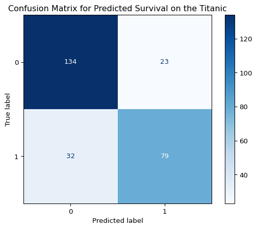
The confusion matrix above shows the breakdown of correct and incorrect predictions. The top-left box shows true negatives (correctly predicted did not survive), the bottom-right shows true positives (correctly predicted survived), and the off-diagonal boxes show our errors: false positives (top-right) and false negatives (bottom-left). This breakdown helps us understand not just how often our model is wrong, but how it’s wrong, which is important for deciding whether the model is good enough for real-world use.
Our model has a slightly higher number of false negatives, which suggests it is undervaluing the probability of some passengers surviving. Our next steps would be understanding the observations where our model fails (perhaps it struggles with the rows that had missing age values?), and iterating on this workflow to improve our model’s performance.
Summary
In this session, we’ve introduced machine learning conceptually and demonstrated a basic supervised learning workflow. Machine learning allows us to build systems that learn patterns from data to make predictions at scale, handling complexity that would overwhelm traditional rules-based systems or simple statistical approaches.
The workflow we followed is the foundation of most supervised learning tasks: get labeled data, split it into training and testing sets, train a model on the training data, make predictions on the test data, and evaluate performance. This split between training and testing is critical because it gives us an honest assessment of how the model performs on data it hasn’t seen before. We also looked at how to evaluate model performance. There are many ways we can build on this workflow to make it more robust and improve model performance.
What we haven’t covered yet is how different models actually learn, why you might choose one model over another, and how to improve performance through feature engineering and hyperparameter tuning. We also haven’t explored other types of machine learning beyond supervised learning, or the full workflow that takes a model from development to deployment. These topics will be covered in the futures, building on the foundations we’ve laid out here.
Footnotes
For example, a rules-based system that classifies patients by their risk-levels might identify a patient over the age of 65 with diabetes and apply a flag to their record that tells clinicians that the patient is high-risk.↩︎
Structured data, also known as tabular data, is any data that can easily fit into a table, with columns representing variables and rows representing different observations.↩︎
Replacing missing values with the mean or median, or dropping missing values entirely, is generally a bad strategy that can have a significant negative impact on your model. However, we are using the median here for the sake of simplicity.↩︎
We will look at other metrics and when we should use them in the future.↩︎