Functions & Functional Programming

This session is the third in a series of programming fundamentals. The concepts here can feel abstract at first, but they are a big part of how Python code is structured in real projects. By the end, you’ll see how functions make code shorter, cleaner, and easier to re-use.

The below slides aim to provide an introduction to these concepts and the way we can use them.

Slides

Use the left ⬅️ and right ➡️ arrow keys to navigate through the slides below. To view in a separate tab/window, follow this link.

What are Functions?

A function is just a reusable set of instructions that takes input, does something with it, and gives you a result.

If you’ve used Excel, you already use functions all the time. For example, SUM(A1:A10) or VLOOKUP(…). You give them arguments (the input), they process it, and they return an output. If you’ve used SQL, it’s the same idea. COUNT(*), ROUND(price, 2), or UPPER(name) are functions. They save you from writing the same logic over and over, and they keep code tidy.

In Python, functions work the same way, but you can also write your own custom ones, so instead of just using what is built-in, you can create tools that do exactly what you need.

Simple Built-In & User-Defined Functions

Python already has many built-in functions which makes the language more functional.

Print Statements

The print() function sends output to the screen. It’s often the first Python function you use.

print("Hello, World!")

Hello, World!

Comparing Operations

We’ll compare how to do things “manually” with loops vs. using Python’s built-in (or imported) functions. This shows how functions save time and reduce code.

Length

We can count the number of items in a list using a for loop.

values = [10, 20, 30, 40, 50]

length_manual = 0
for _ in values:
    length_manual += 1
print("Length:", length_manual)

Length: 5

However, it is much faster to just use len() instead.

print("Length:", len(values))

Length: 5

Sum

We can also sum the value of all the numbers in our values object.

total_manual = 0
for val in values:
    total_manual += val
print("Sum:", total_manual)

Sum: 150

Or we can use sum().

print("Sum:", sum(values))

Sum: 150

Mean

Finally, we can manually calculate the mean of our list of values by summing them and then dividing by the length of the list.

total_for_mean = 0
total_length = 0

for val in values:
    total_for_mean += val

for val in values:
    total_length += 1

mean_manual = total_for_mean / total_length
print("Mean:", mean_manual)

Mean: 30.0

Or we can import numpy and use np.mean().

import numpy as np

values = [10, 20, 30, 40, 50]
print("Mean:", np.mean(values))

Mean: 30.0

Combining Operations

We can create our own functions to group multiple calculations. The function below takes two numbers and returns a sentence describing their sum, difference, and product.

def summarise_numbers(a, b):

    total = a + b
    difference = a - b
    product = a * b
    return (
        f"The sum of {a} and {b} is {total}, "
        f"the difference is {difference}, "
        f"and their product is {product}."
    )

summarise_numbers(10, 5)

'The sum of 10 and 5 is 15, the difference is 5, and their product is 50.'

To illustrate how functions work, we can break them down step-by-step. def summarise_numbers(a, b) is the function header. def states that you are defining a function, summarise_numbers is the function name, and (a, b) is the input parameter (the numbers we are summarising). The function body (the indented code below the header) defines the steps the function should take, and the return statement declares the output from the function.

Exploring Data with Functions

We can use functions to explore an entire dataset quickly and efficiently, where a manual process would require a lot of repetition.

Setup

First, we will import all of the packages we need.

import pandas as pd
import numpy as np
import matplotlib.pyplot as plt
import seaborn as sns
import re

from sklearn.datasets import fetch_california_housing

sns.set_theme(style="whitegrid")

Import Data

We can then import the California housing dataset and store it in housing_raw, before previewing the housing_raw object.

housing_raw = fetch_california_housing(as_frame=True).frame
housing_raw.head()

	MedInc	HouseAge	AveRooms	AveBedrms	Population	AveOccup	Latitude	Longitude	MedHouseVal
0	8.3252	41.0	6.984127	1.023810	322.0	2.555556	37.88	-122.23	4.526
1	8.3014	21.0	6.238137	0.971880	2401.0	2.109842	37.86	-122.22	3.585
2	7.2574	52.0	8.288136	1.073446	496.0	2.802260	37.85	-122.24	3.521
3	5.6431	52.0	5.817352	1.073059	558.0	2.547945	37.85	-122.25	3.413
4	3.8462	52.0	6.281853	1.081081	565.0	2.181467	37.85	-122.25	3.422

Preprocess Data

We’ll make a helper function to convert text to snake_case (lowercase with underscores). This is a common style for column names.

def to_snake_case(s: str) -> str:
    """
    Convert a given string to snake_case.
    """
    s = s.strip()  # remove leading/trailing spaces
    s = re.sub(r'[\s-]+', '_', s)  # replace spaces and hyphens with underscores
    s = re.sub(r'(?<=[a-z])(?=[A-Z])', '_', s)  # add underscore before capital letters
    s = re.sub(r'[^a-zA-Z0-9_]', '', s)  # remove anything not letter, number, or underscore
    return s.lower()  # make everything lowercase

This function has the same basic structure as the function we defined earlier, but with some additional information that is good practice for writing reproducible code. In the function header, the input (s: str) includes the input parameter s and a type-hint starting that s should be a string. The -> str immediately after states that the function will return a string. The triple-quoted text just below the function header describes what the function does. You can also include what the function expects and what it returns.

Next, we can create a function that cleans our dataset, including the to_snake_case function as a step in the process. The other step is to drop all NAs and duplicates.

def preprocess_data(df: pd.DataFrame) -> pd.DataFrame:
    """
    Preprocess a dataframe by cleaning and standardizing column names.
    """
    df = df.dropna().drop_duplicates().copy()  # remove missing rows and duplicates
    df.columns = [to_snake_case(col) for col in df.columns]  # rename columns to snake_case
    return df  # return cleaned dataframe

We can then apply this to our dataset.

df = preprocess_data(housing_raw)
df.head()

	med_inc	house_age	ave_rooms	ave_bedrms	population	ave_occup	latitude	longitude	med_house_val
0	8.3252	41.0	6.984127	1.023810	322.0	2.555556	37.88	-122.23	4.526
1	8.3014	21.0	6.238137	0.971880	2401.0	2.109842	37.86	-122.22	3.585
2	7.2574	52.0	8.288136	1.073446	496.0	2.802260	37.85	-122.24	3.521
3	5.6431	52.0	5.817352	1.073059	558.0	2.547945	37.85	-122.25	3.413
4	3.8462	52.0	6.281853	1.081081	565.0	2.181467	37.85	-122.25	3.422

Visualise Distributions

A great way to use functions for exploratory data analysis is for visualing multiple columns at once. If we visualise every column manually, this would require a lot of code. However, we can write a single function that returns a plot for every relevant column in a single figure.

Below is a function for plotting a histogram for each numeric column in a single figure.

def plot_numeric_columns(df: pd.DataFrame) -> None:

    """
    plot histograms for all numeric columns in one figure with subplots.
    """
    
    numeric_cols = df.select_dtypes(include=[np.number]).columns  # get numeric column names
    n = len(numeric_cols)  # count how many numeric columns there are
    if n == 0: # if there are no numeric columns  
        print("no numeric columns found") # tell the user
        return # and stop the function

    # determine how many plots per row (max 3)
    ncols = min(n, 3)  # number of columns in subplot grid
    nrows = (n + ncols - 1) // ncols  # number of rows in subplot grid (ceiling division)
    fig, axes = plt.subplots(nrows, ncols, figsize=(6 * ncols, 4 * nrows))  # create figure and axes
    if n == 1:  # if only one numeric column
        axes = [axes]  # put single axis in a list for consistency
    else:
        axes = axes.flatten()  # flatten 2d array of axes into 1d list

    for ax, col in zip(axes, numeric_cols):  # loop through axes and column names
        ax.hist(df[col], bins=20, edgecolor="black")  # draw histogram for column
        ax.set_xlabel(col)  # set x-axis label
        ax.set_ylabel("")  # remove y-axis label

    # remove any extra empty plots
    for ax in axes[len(numeric_cols):]:  # loop over unused axes
        fig.delaxes(ax)  # delete unused subplot

    plt.tight_layout()  # adjust layout so plots don't overlap
    plt.show()  # display the plots

And then we can run this function on our California housing dataset.

plot_numeric_columns(df)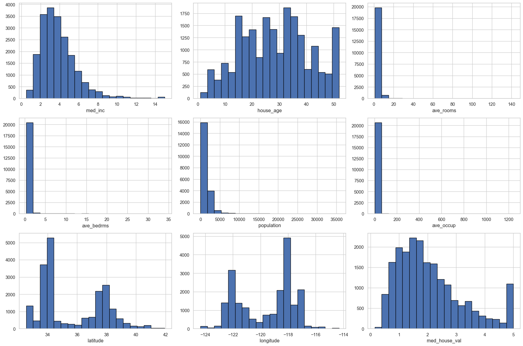

We can do the same for categorical columns, using bar charts.

def plot_categorical_columns(df: pd.DataFrame) -> None:
    
    """
    plot bar charts for all categorical columns in one figure with subplots.
    """
    
    cat_cols = df.select_dtypes(exclude=[np.number]).columns  # get non-numeric column names
    n = len(cat_cols)  # count how many categorical columns there are
    if n == 0:  # if there are no categorical columns
        print("no categorical columns found")  # tell the user
        return  # and stop the function

    # determine how many plots per row (max 3)
    ncols = min(n, 3)  # number of columns in subplot grid
    nrows = (n + ncols - 1) // ncols  # number of rows in subplot grid (ceiling division)
    fig, axes = plt.subplots(nrows, ncols, figsize=(6 * ncols, 4 * nrows))  # create figure and axes
    if n == 1:  # if only one categorical column
        axes = [axes]  # put single axis in a list for consistency
    else:
        axes = axes.flatten()  # flatten 2d array of axes into 1d list

    for ax, col in zip(axes, cat_cols):  # loop through axes and column names
        df[col].value_counts().plot(kind="bar", ax=ax, edgecolor="black")  # draw bar chart
        ax.set_xlabel(col)  # set x-axis label
        ax.set_ylabel("")  # remove y-axis label

    # remove any extra empty plots
    for ax in axes[len(cat_cols):]:  # loop over unused axes
        fig.delaxes(ax)  # delete unused subplot

    plt.tight_layout()  # adjust layout so plots don't overlap
    plt.show()  # display the plots

However, there are no categorical columns in this dataset¹.

plot_categorical_columns(df)

no categorical columns found

Summary

Functions let you package steps into reusable, predictable tools. You will have used functions before in other settings, and when writing Python code you will regularly encounter built-in functions and functions imported from packages. The more you work in Python, the more you’ll see yourself building small helper functions to avoid repeating code.

Exercises

1. Write a function that returns the maximum and minimum values in a list.

Solution

def min_max(lst):
    return min(lst), max(lst)

min_max([4, 1, 9])

(1, 9)

2. Modify summarise_numbers to also return the division result (a / b).

Solution

def summarise_numbers(a, b):
    total = a + b
    difference = a - b
    product = a * b
    division = a / b
    return total, difference, product, division

summarise_numbers(5, 10)

(15, -5, 50, 0.5)

3. Write a function that counts how many even numbers are in a list.

Hint: This requires using a ‘modulo operator’².

Solution

def count_evens(lst):
    return sum(1 for x in lst if x % 2 == 0)

values = [1, 2, 3, 4, 5]
count_evens(values)

2

For the next three questions, you can use this sample dataset:

sample_df = pd.DataFrame({
    "Name": np.random.choice(["Alice", "Bob", "Charlie", "John"], size=20),
    "Department": np.random.choice(["HR", "IT", "Finance"], size=20),
    "Age": np.random.randint(21, 60, size=20),
    "Salary": np.random.randint(30000, 80000, size=20),
    "Years_at_Company": np.random.randint(1, 20, size=20)
})

4. Create a function that takes a dataframe and returns only columns with numeric data.

Solution

def select_numeric(df):
    return df.select_dtypes(include=[np.number])

select_numeric(sample_df)

	Age	Salary	Years_at_Company
0	45	40356	16
1	42	55202	4
2	38	31157	16
3	22	67908	6
4	44	47844	14
5	37	33289	15
6	34	36306	10
7	21	72968	18
8	34	47750	6
9	37	79227	16
10	52	48552	8
11	51	78211	8
12	26	61080	14
13	42	46634	5
14	34	61960	14
15	32	31033	6
16	44	63980	9
17	41	70280	1
18	38	34418	8
19	48	42661	18

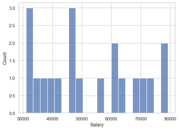
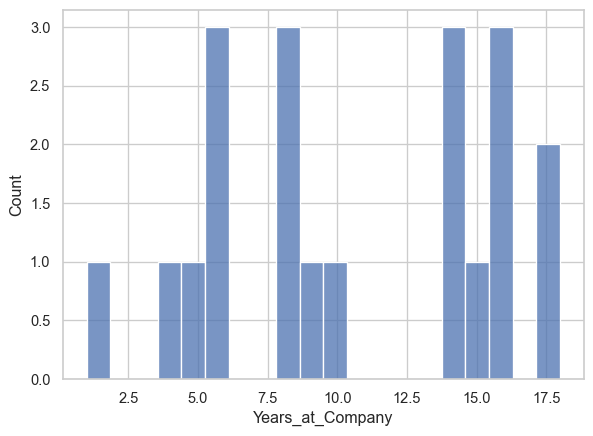
5. Rewrite plot_numeric_columns so it uses seaborn’s histplot instead of matplotlib’s hist.

Solution

def plot_numeric_columns(df):
    numeric_cols = df.select_dtypes(include=[np.number]).columns
    for col in numeric_cols:
        sns.histplot(df[col], bins=20)
        plt.show()

plot_numeric_columns(sample_df)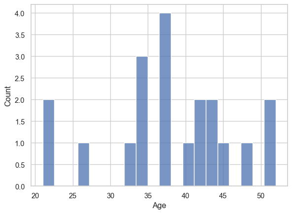

6. Write a function that converts all string columns in a dataframe to lowercase.

Solution

def lowercase_strings(df):
    for col in df.select_dtypes(include=['object']):
        df[col] = df[col].str.lower()
    return df

lowercase_strings(sample_df)

	Name	Department	Age	Salary	Years_at_Company
0	bob	finance	45	40356	16
1	bob	hr	42	55202	4
2	bob	finance	38	31157	16
3	john	hr	22	67908	6
4	charlie	hr	44	47844	14
5	john	it	37	33289	15
6	john	hr	34	36306	10
7	john	it	21	72968	18
8	bob	it	34	47750	6
9	bob	it	37	79227	16
10	charlie	it	52	48552	8
11	john	finance	51	78211	8
12	charlie	hr	26	61080	14
13	john	finance	42	46634	5
14	bob	finance	34	61960	14
15	john	it	32	31033	6
16	charlie	it	44	63980	9
17	alice	it	41	70280	1
18	bob	finance	38	34418	8
19	john	hr	48	42661	18

Footnotes

1. This is just here as a demonstration of how you would do this with categorical columns, and to show what it would look like if the function cannot find relevant columns and stops early.

2. If you don’t know what a modulo operator is (totally understandable), you can search this online and it will likely help you find the answer to this question. It is always okay (encouraged, even) to search for answers to code questions online.