Regression Fundamentals: Introduction to Linear Regression
This is the third session in our regression foundations series. Previous sessions discussed how to evaluate the differences between samples and the relationships between pairs of variables. This session will focus on bringing all of that together in order to make more precise inferences and predictions using data.
We’ll continue using the Palmer Penguins dataset to build intuition for regression concepts, then apply these methods to understand what drives penguin body mass and how we can predict it from other physical characteristics.
Slides
Use the left ⬅️ and right ➡️ arrow keys to navigate through the slides below. To view in a separate tab/window, follow this link.
What is Regression?
Regression is a method for modelling the relationship between one or more explanatory variables (or predictors) and an outcome of interest. The goal of regression is to find a function that predicts the outcome from the predictors.
Regression is incredibly flexible in both approach and application. It can fit to all kinds of data problem and can be used for descriptive, explanatory, and predictive analysis. For this reason, it is a foundational tool in statistics and data science.
Why Build Models?
In our previous sessions, we compared groups (4/20 vs other days) and examined relationships (penguin flipper length vs body mass). But both approaches had limitations: group comparisons can’t handle continuous predictors, and correlation only measures linear association between two variables at a time.
Regression bridges these gaps. It lets us:
Quantify how much \(Y\) changes when \(X\) increases by one unit.
Include multiple predictors simultaneously.
Make predictions for new observations.
Test specific hypotheses about relationships.
Account for confounding variables.
Instead of just knowing flipper length and body mass are correlated, we can say that each additional millimeter increase in flipper length predicts an \(X\) increase in body mass. And we can go much further than this, controlling for environment, treating species as a grouping structure in the data, or facotoring in non-linearity. With regression, the possibilities are practically endless.
From Association to Inference & Prediction
Correlation tells us variables move together. Regression tells us by how much and in what direction, and gives us the tools to make inferences and predictions.
Consider these questions that regression can answer but correlation cannot:
If a penguin’s flipper is 200mm, what body mass do we predict?
How does the flipper-mass relationship differ between species?
What’s our uncertainty around these predictions?
Which variables matter most for predicting body mass?
The Linear Regression Model
The most common type of regression model, and the foundation from which so many other types of regression model are built, is linear regression. Linear regression assumes the relationship between the predictors and the outcome are linear, meaning that when predictors change in value the outcome changes by a constant amount. Visually, this just means fitting a straight line through data. For example, if you are paid £10 an hour, your pay increases by exactly £10 for each additional hour worked. This is a linear relationship.
If you have a predictor \(X\) and an outcome \(Y\), linear regression finds the path through the data that best fits these points, otherwise known as the “line of best fit”. This works by finding a line that passes through the data with the minimum amount of prediction error, which is the observed value minus the predicted value for each data pint (and is oftn referred to as the residual). The most common way for calculating the line of best fit is called Ordinary Least Squares (OLS)[^OLS].
Calculating the Line of Best fit Using OLS (Click to Expand)
Ordinary Least Squares Estimation
We won’t spend too much time on OLS in this session, but the method it uses for calculating the line of best fit is as follows:
Calculate the residual for each observation (the actual value minus the predicted value).
Square the residuals (so that positive and negative errors do not cancel each other out).
Sum the squared residuals, sometimes called the Residual Sum of Squares (RSS).
Find the line that produces the smallest RSS.
The formula for a simple linear regression model, predicting \(Y\) with one predictor \(X\):
This breaks the problem down into three components, and estimates two parameters:
\(\beta_1\) - The slope, estimating the effect that \(X\) has on the outcome, \(Y\).
\(\beta_0\) - The intercept, estimating the average value of \(Y\) when \(X = 0\).
\(\epsilon\) - The error term, capturing the remaining variance in the outcome \(Y\) that is not explained by the rest of the model.
Don’t worry if this is intimidating at first. The main thing you need to remember is that this equation is just fitting a straight line through the data.
The regression line represents our best guess of the true relationship, and the scatter around the line represents uncertainty.
Building Our First Model
Import & Prepare Data
import pandas as pdimport numpy as npimport matplotlib.pyplot as pltimport seaborn as snsfrom scipy import statsimport statsmodels.api as smfrom sklearn.linear_model import LinearRegressionfrom sklearn.metrics import r2_score# load penguins dataurl ='https://raw.githubusercontent.com/rfordatascience/tidytuesday/main/data/2025/2025-04-15/penguins.csv'penguins_raw = pd.read_csv(url)# clean datadf = penguins_raw.dropna()df.head()
species
island
bill_len
bill_dep
flipper_len
body_mass
sex
year
0
Adelie
Torgersen
39.1
18.7
181.0
3750.0
male
2007
1
Adelie
Torgersen
39.5
17.4
186.0
3800.0
female
2007
2
Adelie
Torgersen
40.3
18.0
195.0
3250.0
female
2007
4
Adelie
Torgersen
36.7
19.3
193.0
3450.0
female
2007
5
Adelie
Torgersen
39.3
20.6
190.0
3650.0
male
2007
Visualising the Relationship
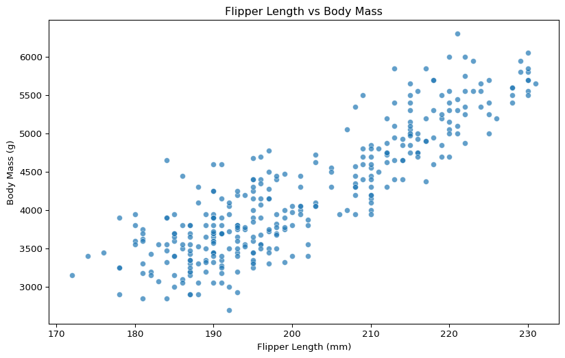
plt.figure(figsize=(10, 6))sns.scatterplot(data=df, x='flipper_len', y='body_mass', alpha=0.7)plt.title('Flipper Length vs Body Mass')plt.xlabel('Flipper Length (mm)')plt.ylabel('Body Mass (g)')plt.show()
The relationship looks strongly linear and positive. This is a good candidate for linear regression.
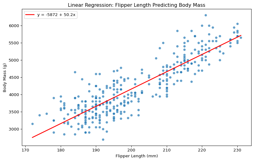
The intercept (\(\beta_0\)) = -5872.1g. The intercept tells us the predicted body mass when flipper length is 0mm. This intercept value is not meaningful because a flipper length of zero is implausible and ultimately nonsensical (if they have flippers, they must be longer than 0mm)1, but we need the intercept to fit the model.
The slope (\(\beta_1\)) = 50.2g/mm. The slope tells us that each additional mm increase in flipper length predicts ~50g increase in body mass.
Visualising the Fitted Line
We can add the fitted line to our scatterplot and use this to make predictions by tracing the flipper length from which we want to predict body mass and then finding the body mass at that value.
Using a fitted line to make predictions is imprecise. Instead, we can use the linear regression formula detailed earlier to predict penguin body mass from flipper length. We just have to plug in the intercept and slope into the formula, along with the flipper length we want to predict from, and this will give us the predicted body mass.
# predict body mass for different flipper lengthsnew_flipper_lengths = np.array([[190], [200], [210], [220]])predictions = model.predict(new_flipper_lengths)prediction_df = pd.DataFrame({'Flipper Length (mm)': new_flipper_lengths.flatten(),'Predicted Body Mass (g)': predictions.round(0)})print("Predictions for new observations:")print(prediction_df)
Predictions for new observations:
   Flipper Length (mm)  Predicted Body Mass (g)
0                  190                   3657.0
1                  200                   4159.0
2                  210                   4660.0
3                  220                   5162.0
Statistical Inference
So far we’ve focused on prediction. But regression also lets us make inferences about the relationship between variables.
# use statsmodels for explanatory modelsX_sm = sm.add_constant(df['flipper_len']) # add intercept columnmodel_sm = sm.OLS(df['body_mass'], X_sm).fit()print(model_sm.summary().tables[1])
When we are interested in explaining rather than predicting, the coefficient (coef) is what matters most. This is the intercept and slope values we calculated earlier. The coefficients tell us the size of the effect observed in the data. If you want to explain the relationship between variables, the effect size is the most important part of the model.
The other outputs are useful for understanding how well your model fits to the data and how certain the model is about the estimates. The standard error (std error) tells us how much the actual values vary around the fitted line, quantifying uncertainty. The 95% confidence intervals ([0.025 & 0.975]) are another way of expressing this idea. They effectively show a range of plausible coefficient values.
Finally, the t-statistic (t) is a test statistic2 and the p-value (P>|t|) is the probability of observing an effect as large (or larger) as observed in the data if there was actually no relationship between flipper length and body mass (and if the assumptions of the model are valid). You can think of the p-value as an expression of how surprising it would be to see a coefficient as large as the one we found if there wasn’t actually a relationship between flipper length and body mass.
Summary
Linear regression transforms correlation into a predictive and explanatory tool. We can quantify relationships and make predictions. Our penguin model shows that flipper length strongly predicts body mass, with each additional mm corresponding to ~50g increase in weight.
The key insights from regression go beyond simple correlation: we can make specific predictions, quantify uncertainty, and begin to understand the mechanisms behind relationships. However, real-world relationships are often more complex than simple linear models can capture.
In the next session, we will go into greater detail about the implementation of linear regression, looking at how we fit models, their assumptions, and how we interpret, present, and communicate our outputs.
Footnotes
For explanatory models, it is generally best-practice to transform the data so that the intercept is meaningful. For example, subtracting the mean flipper length from each observation (otherwise known as centering) so that the zero value represents the average flipper length and the intercept represents the average body mass for the average flipper length.↩︎
We will not discuss test statistics in detail here, but they are standardised measures of how unusual your results are. It is used to calculate the p-value. The t-statistic is the coefficient divided by its standard error.↩︎