Regression Fundamentals: Implementing Linear Regression

In the previous session, we explored what linear regression is, how it works conceptually, and why it’s such a powerful tool. We saw how regression finds the line of best fit by minimising prediction errors, and we understood the core components: intercepts, slopes, and residuals.

Now it’s time to put that theory into practice. In this session, we’ll learn how to actually build regression models in Python, interpret their outputs, check whether our models are valid, and generate insights from them.

We’ll cover two main approaches to regression in Python:

scikit-learn - Focused on prediction and machine learning workflows.
statsmodels - Focused on statistical inference and hypothesis testing.

Let’s get started by loading our data and packages.

import pandas as pd
import numpy as np
import matplotlib.pyplot as plt
import seaborn as sns


from sklearn.linear_model import LinearRegression
from sklearn.metrics import r2_score, mean_squared_error
import statsmodels.api as sm
import statsmodels.formula.api as smf

import warnings
warnings.filterwarnings('ignore')

# set visualisation style
sns.set_theme(style="whitegrid")
plt.rcParams['figure.figsize'] = (10, 6)

# load palmer penguins data
url = 'https://raw.githubusercontent.com/rfordatascience/tidytuesday/main/data/2025/2025-04-15/penguins.csv'
df = pd.read_csv(url)

# drop missing values for simplicity
df = df.dropna()

Building Predictive Models Using Scikit-Learn

scikit-learn (sklearn) is Python’s most popular library for machine learning. Its regression tools are designed for building predictive models, and it is optimised for generalising well on new data.

Simple Linear Regression

A simple linear regression has one predictor variable. Let’s predict body mass from flipper length.

# prepare the data
# sklearn requires 2D arrays for X (predictors) and 1D arrays for y (outcome)
X = df[['flipper_len']]  # double brackets create a dataframe
y = df['body_mass']       # single bracket creates a series

# create and fit the model
model = LinearRegression()
model.fit(X, y)

# get the intercept
intercept = model.intercept_
print(f"Intercept = {intercept:.2f}g")

# get the slope
slope = model.coef_[0]
print(f"Slope = {slope:.2f}g per mm")

Intercept = -5872.09g
Slope = 50.15g per mm

The fitted model object contains everything we need: coefficients, predictions, and model performance metrics.

The intercept (\(\beta_0\)) = -5872.1g. The intercept tells us the predicted body mass when flipper length is 0mm. This intercept value is not meaningful because a flipper length of zero is implausible and ultimately nonsensical (if they have flippers, they must be longer than 0mm)¹, but we need the intercept to fit the model.

The slope (\(\beta_1\)) = 50.2g/mm. The slope tells us that each additional mm increase in flipper length predicts ~50g increase in body mass.

Making Predictions

Once we have a fitted model, we can use it to predict body mass for any flipper length.

# predict body mass for all penguins in our dataset
y_pred = model.predict(X)

# add predictions to our dataframe
df['predicted_mass'] = y_pred
df['residual'] = df['body_mass'] - df['predicted_mass']

# look at some predictions
print("Sample predictions:")
print(df[['flipper_len', 'body_mass', 'predicted_mass', 'residual']].head(10))

Sample predictions:
    flipper_len  body_mass  predicted_mass    residual
0         181.0     3750.0     3205.648453  544.351547
1         186.0     3800.0     3456.414782  343.585218
2         195.0     3250.0     3907.794176 -657.794176
4         193.0     3450.0     3807.487644 -357.487644
5         190.0     3650.0     3657.027846   -7.027846
6         181.0     3625.0     3205.648453  419.351547
7         195.0     4675.0     3907.794176  767.205824
12        182.0     3200.0     3255.801719  -55.801719
13        191.0     3800.0     3707.181112   92.818888
14        198.0     4400.0     4058.253974  341.746026

We can plot the predictions too.

# plot
fig, ax = plt.subplots(figsize=(10, 6))
sns.scatterplot(data=df, x='flipper_len', y='body_mass', color='#005EB8', alpha=0.5, ax=ax, label='Observed')
sns.scatterplot(data=df, x='flipper_len', y='predicted_mass', color='red', alpha=0.5, ax=ax, label='Predicted')

ax.set_xlabel('Flipper Length (mm)')
ax.set_ylabel('Body Mass (g)')
ax.set_title('Observed vs Predicted Body Mass')
ax.legend()

plt.tight_layout()
plt.show()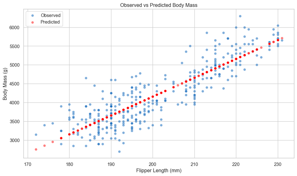

We can also predict for new data.

# predict for hypothetical penguins
new_penguins = pd.DataFrame({
    'flipper_len': [180, 200, 220]
})

new_predictions = model.predict(new_penguins)

print("\nPredictions for new penguins:")
for flipper, mass in zip(new_penguins['flipper_len'], new_predictions):
    print(f"Flipper length: {flipper}mm --> Predicted mass: {mass:.0f}g")


Predictions for new penguins:
Flipper length: 180mm --> Predicted mass: 3155g
Flipper length: 200mm --> Predicted mass: 4159g
Flipper length: 220mm --> Predicted mass: 5162g

Model Performance Metrics

An important part of predictive modelling is evaluation. We need to test how well our model is performing! sklearn provides a wide variety of metrics for assessing model performance. We will look at \(\text{R}^2\) and RMSE.

# r-squared: proportion of variance explained
r2 = r2_score(y, y_pred)

# root mean squared error: average prediction error in grams
rmse = np.sqrt(mean_squared_error(y, y_pred))

The \(\text{R}^2\) = 0.76, which suggests that flipper length explains a significant amount of the variance in penguin body mass, while the RMSE indicates that the average prediction error is 392.16g. This means that predictions are, on average, off by 392.16g.

There is no rule of thumb or minimum threshold for good prediction error. It all depends on what you are trying to predict and what is needed for predictions to be useful. Another model trying to predict something completely different might have much larger prediction errors but this still be useful in context. It is always necessary to judge a model in context.

Multiple Linear Regression

Now let’s add more predictors. Multiple regression lets us understand the effect of each variable while controlling for the others.

# add bill length and bill depth as predictors
X_multi = df[['flipper_len', 'bill_len', 'bill_dep']]
y = df['body_mass']

# fit the model
model_multi = LinearRegression()
model_multi.fit(X_multi, y)

# extract coefficients
print("Multiple regression coefficients:")
print(f"Intercept: {model_multi.intercept_:.2f}g")
for name, coef in zip(X_multi.columns, model_multi.coef_):
    print(f"  {name}: {coef:.2f}g per unit")

# compare model performance
y_pred_multi = model_multi.predict(X_multi)
r2_multi = r2_score(y, y_pred_multi)
rmse_multi = np.sqrt(mean_squared_error(y, y_pred_multi))

print(f"\nModel comparison:")
print(f"Simple model (flipper only):   R² = {r2:.3f}, RMSE = {rmse:.1f}g")
print(f"Multiple model (three vars):   R² = {r2_multi:.3f}, RMSE = {rmse_multi:.1f}g")

Multiple regression coefficients:
Intercept: -6445.48g
  flipper_len: 50.76g per unit
  bill_len: 3.29g per unit
  bill_dep: 17.84g per unit

Model comparison:
Simple model (flipper only):   R² = 0.762, RMSE = 392.2g
Multiple model (three vars):   R² = 0.764, RMSE = 390.6g

Adding bill measurements improves our model slightly. Each predictor contributes information beyond what the others provide.

Building Inferential Models Using Statsmodels

statsmodels is designed for statistical inference². It provides detailed output about uncertainty, hypothesis tests, and model diagnostics. This is what you want when your goal is understanding relationships rather than pure prediction.

Adding predictors is straightforward with the formula interface.

# multiple regression with formula
model_sm = smf.ols('body_mass ~ flipper_len + bill_len + bill_dep', data=df).fit()

print(model_sm.summary())

                            OLS Regression Results                            
==============================================================================
Dep. Variable:              body_mass   R-squared:                       0.764
Model:                            OLS   Adj. R-squared:                  0.762
Method:                 Least Squares   F-statistic:                     354.9
Date:                Thu, 06 Nov 2025   Prob (F-statistic):          9.26e-103
Time:                        13:30:25   Log-Likelihood:                -2459.8
No. Observations:                 333   AIC:                             4928.
Df Residuals:                     329   BIC:                             4943.
Df Model:                           3                                         
Covariance Type:            nonrobust                                         
===============================================================================
                  coef    std err          t      P>|t|      [0.025      0.975]
-------------------------------------------------------------------------------
Intercept   -6445.4760    566.130    -11.385      0.000   -7559.167   -5331.785
flipper_len    50.7621      2.497     20.327      0.000      45.850      55.675
bill_len        3.2929      5.366      0.614      0.540      -7.263      13.849
bill_dep       17.8364     13.826      1.290      0.198      -9.362      45.035
==============================================================================
Omnibus:                        5.596   Durbin-Watson:                   1.982
Prob(Omnibus):                  0.061   Jarque-Bera (JB):                5.469
Skew:                           0.312   Prob(JB):                       0.0649
Kurtosis:                       3.068   Cond. No.                     5.44e+03
==============================================================================

Notes:
[1] Standard Errors assume that the covariance matrix of the errors is correctly specified.
[2] The condition number is large, 5.44e+03. This might indicate that there are
strong multicollinearity or other numerical problems.

The statsmodels summary is dense but incredibly informative. Here’s what matters most.

coef - The estimated effect size of each variable holding the others constant
std err - Uncertainty in the estimate
t - Test statistic (coef / std err)
P>|t| - p-value for null hypothesis that coefficient = 0
[0.025, 0.975] - 95% confidence interval

Focus on effect sizes first, then uncertainty. The coefficient tells you the magnitude of the relationship. The confidence interval tells you how precisely we’ve estimated it. Don’t obsess over \(\text{R}^2\)³ or p-values. The most important part of the model is the coefficients.

The p-value is useful as a diagnostic, indicating whether you have enough data, but it doesn’t tell you whether the effect is meaningful or important.

We can also produce a simpler regression table, if the above is overwhelming.

# extract just the coefficients table
print(model_sm.summary().tables[1])

===============================================================================
                  coef    std err          t      P>|t|      [0.025      0.975]
-------------------------------------------------------------------------------
Intercept   -6445.4760    566.130    -11.385      0.000   -7559.167   -5331.785
flipper_len    50.7621      2.497     20.327      0.000      45.850      55.675
bill_len        3.2929      5.366      0.614      0.540      -7.263      13.849
bill_dep       17.8364     13.826      1.290      0.198      -9.362      45.035
===============================================================================

Styled Tables (Click to Expand)

For presentations and reports, we can create publication-ready tables.

from great_tables import GT, md, html
from great_tables import loc, style

# fit three models for comparison
model1 = smf.ols('body_mass ~ flipper_len', data=df).fit()
model2 = smf.ols('body_mass ~ flipper_len + bill_len + bill_dep', data=df).fit()
model3 = smf.ols('body_mass ~ flipper_len + bill_len + bill_dep + C(species)', data=df).fit()

# create a dataframe with model results
results_df = pd.DataFrame({
    'Variable': ['Intercept', 'Flipper Length', 'Bill Length', 'Bill Depth', 
                 'Chinstrap', 'Gentoo'],
    'Model 1': [
        f"{model1.params['Intercept']:.1f}",
        f"{model1.params['flipper_len']:.2f}***",
        '—', '—', '—', '—'
    ],
    'Model 2': [
        f"{model2.params['Intercept']:.1f}",
        f"{model2.params['flipper_len']:.2f}***",
        f"{model2.params['bill_len']:.2f}***",
        f"{model2.params['bill_dep']:.2f}",
        '—', '—'
    ],
    'Model 3': [
        f"{model3.params['Intercept']:.1f}",
        f"{model3.params['flipper_len']:.2f}***",
        f"{model3.params['bill_len']:.2f}***",
        f"{model3.params['bill_dep']:.2f}**",
        f"{model3.params['C(species)[T.Chinstrap]']:.1f}***",
        f"{model3.params['C(species)[T.Gentoo]']:.1f}***"
    ]
})

# add model statistics
stats_df = pd.DataFrame({
    'Variable': ['', 'N', 'R²', 'Adj. R²', 'AIC'],
    'Model 1': ['', f"{int(model1.nobs)}", f"{model1.rsquared:.3f}", 
                f"{model1.rsquared_adj:.3f}", f"{model1.aic:.1f}"],
    'Model 2': ['', f"{int(model2.nobs)}", f"{model2.rsquared:.3f}", 
                f"{model2.rsquared_adj:.3f}", f"{model2.aic:.1f}"],
    'Model 3': ['', f"{int(model3.nobs)}", f"{model3.rsquared:.3f}", 
                f"{model3.rsquared_adj:.3f}", f"{model3.aic:.1f}"]
})

combined_df = pd.concat([results_df, stats_df], ignore_index=True)

# create styled table
table = (
    GT(combined_df)
    .tab_header(
        title="Regression Models Predicting Penguin Body Mass",
        subtitle="Coefficients with significance stars (* p<0.05, ** p<0.01, *** p<0.001)"
    )
    .tab_spanner(
        label="Model Specifications",
        columns=['Model 1', 'Model 2', 'Model 3']
    )
    .tab_style(
        style=style.text(weight="bold"),
        locations=loc.body(rows=[6, 7, 8, 9, 10])
    )
    .tab_style(
        style=style.borders(sides="top", weight="2px"),
        locations=loc.body(rows=[6])
    )
    .cols_align(
        align="center",
        columns=['Model 1', 'Model 2', 'Model 3']
    )
    .cols_align(
        align="left",
        columns=['Variable']
    )
)

table

Variable	Model Specifications
Regression Models Predicting Penguin Body Mass
Coefficients with significance stars (* p<0.05, p<0.01, * p<0.001)
Variable	Model 1	Model 2	Model 3
Intercept	-5872.1	-6445.5	-4282.1
Flipper Length	50.15***	50.76***	20.23***
Bill Length	—	3.29***	39.72***
Bill Depth	—	17.84	141.77**
Chinstrap	—	—	-496.8***
Gentoo	—	—	965.2***

N	333	333	333
R²	0.762	0.764	0.849
Adj. R²	0.761	0.762	0.847
AIC	4926.1	4927.6	4781.7

Adding Categorical Variables

statsmodels handles categorical variables automatically with the formula interface.

# add species as a categorical predictor
# statsmodels automatically creates dummy variables
model_species_sm = smf.ols('body_mass ~ flipper_len + bill_len + bill_dep + C(species)', 
                           data=df).fit()

print(model_species_sm.summary())

                            OLS Regression Results                            
==============================================================================
Dep. Variable:              body_mass   R-squared:                       0.849
Model:                            OLS   Adj. R-squared:                  0.847
Method:                 Least Squares   F-statistic:                     369.1
Date:                Thu, 06 Nov 2025   Prob (F-statistic):          4.22e-132
Time:                        13:30:25   Log-Likelihood:                -2384.8
No. Observations:                 333   AIC:                             4782.
Df Residuals:                     327   BIC:                             4805.
Df Model:                           5                                         
Covariance Type:            nonrobust                                         
===========================================================================================
                              coef    std err          t      P>|t|      [0.025      0.975]
-------------------------------------------------------------------------------------------
Intercept               -4282.0802    497.832     -8.601      0.000   -5261.438   -3302.723
C(species)[T.Chinstrap]  -496.7583     82.469     -6.024      0.000    -658.995    -334.521
C(species)[T.Gentoo]      965.1983    141.770      6.808      0.000     686.301    1244.096
flipper_len                20.2264      3.135      6.452      0.000      14.059      26.394
bill_len                   39.7184      7.227      5.496      0.000      25.501      53.936
bill_dep                  141.7714     19.163      7.398      0.000     104.072     179.470
==============================================================================
Omnibus:                        7.321   Durbin-Watson:                   2.248
Prob(Omnibus):                  0.026   Jarque-Bera (JB):                7.159
Skew:                           0.348   Prob(JB):                       0.0279
Kurtosis:                       3.179   Cond. No.                     6.01e+03
==============================================================================

Notes:
[1] Standard Errors assume that the covariance matrix of the errors is correctly specified.
[2] The condition number is large, 6.01e+03. This might indicate that there are
strong multicollinearity or other numerical problems.

The C() wrapper tells statsmodels to treat species as categorical. The model automatically creates “dummy variables”, which splits the categorical variable into multiple columns, with each column being a binary variable representing a category (where the variable equals one when that category appears in the original column).

When creating the dummy variables, the model drops one category to use it as the reference category against which the other categories are compared. This means that coefficients for those categories tell us how much the outcome variable increases or decreases compared against the reference category that was dropped.

For example, the model specified above uses Adelie penguins as the reference category (it chooses by alphabetical order by default), and the coefficients represent the species effects relative to Adelie penguins.

print("\nSpecies effects relative to Adelie:")
for var in model_species_sm.params.index:
    if 'species' in var:
        coef = model_species_sm.params[var]
        ci = model_species_sm.conf_int().loc[var]
        species = var.split('[T.')[1].rstrip(']')
        print(f"{species:12s}: {coef:7.0f}g heavier [{ci[0]:7.0f}, {ci[1]:7.0f}]")


Species effects relative to Adelie:
Chinstrap   :    -497g heavier [   -659,    -335]
Gentoo      :     965g heavier [    686,    1244]

Coefficient Plots

Coefficient plots show effect sizes and their uncertainty at a glance.

# extract coefficients and confidence intervals
coefs = model_species_sm.params.drop('Intercept')
conf_int = model_species_sm.conf_int().drop('Intercept')

# create dataframe for plotting
coef_data = pd.DataFrame({
    'Variable': coefs.index,
    'Coefficient': coefs.values,
    'Lower': conf_int[0].values,
    'Upper': conf_int[1].values
})

# plot
fig, ax = plt.subplots(figsize=(10, 6))
sns.scatterplot(data=coef_data, x='Coefficient', y='Variable', s=200, 
                color='#005EB8', ax=ax)
for idx, row in coef_data.iterrows():
    ax.plot([row['Lower'], row['Upper']], [row['Variable'], row['Variable']], 
            color='#005EB8', linewidth=2)
ax.axvline(x=0, color='red', linestyle='--', linewidth=1)
ax.set_xlabel('Coefficient (Effect on Body Mass, g)')
ax.set_title('Coefficient Plot with 95% Confidence Intervals')
plt.tight_layout()
plt.show()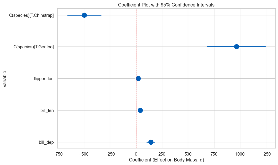

Variables whose CI doesn’t cross zero have effects distinguishable from zero. But remember: focus on effect sizes, not just significance!

Regression Assumptions and Diagnostics

Linear regression makes several assumptions. When these hold, OLS gives us the Best Linear Unbiased Estimator (BLUE). When they don’t, we need to either fix the problem⁴ or acknowledge the limitations.

The Gauss-Markov Theorem

Under certain conditions, OLS is BLUE:

Linearity: The relationship between X and Y is linear
Independence: Observations are independent of each other
Homoscedasticity: Variance of errors is constant across X
No perfect multicollinearity: Predictors aren’t perfectly correlated
Exogeneity: Errors have mean zero (no systematic bias)

Additionally, for valid inference (confidence intervals, p-values), we need:

Normality: Errors are normally distributed (or we have a large sample)

Let’s check these assumptions systematically.

Diagnostic Plots

We’ll create a set of diagnostic plots to check our assumptions. First, let’s fit a model to diagnose.

# fit our model with species
model = model_species_sm  # use the statsmodels model from earlier

# get predictions and residuals
df['fitted'] = model.fittedvalues
df['residuals'] = model.resid
df['standardised_residuals'] = model.resid_pearson

1. Residuals vs Fitted (Linearity & Homoscedasticity)

fig, ax = plt.subplots(figsize=(10, 6))
sns.scatterplot(x=df['fitted'], y=df['residuals'], alpha=0.6, ax=ax)
ax.axhline(y=0, color='red', linestyle='--', linewidth=2)
ax.set_xlabel('Fitted Values')
ax.set_ylabel('Residuals')
ax.set_title('Residuals vs Fitted Values')
plt.show()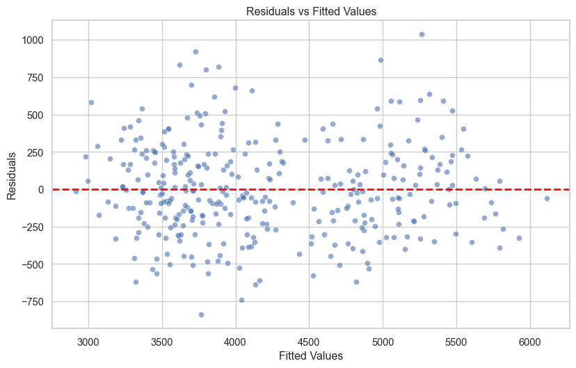

The observations should appear to be randomly scattered around zero, and the spread around zero should be constant across the range of fitted values. If you can see a pattern or trend, this suggests the linearity assumption is violated, and if the observations are funnel-shaped, this suggests that the homoscedasticity assumption is violated.

2. Q-Q Plot (Normality)

from scipy import stats

fig, ax = plt.subplots(figsize=(10, 6))
stats.probplot(df['residuals'], dist="norm", plot=ax)
ax.set_title('Q-Q Plot')
plt.show()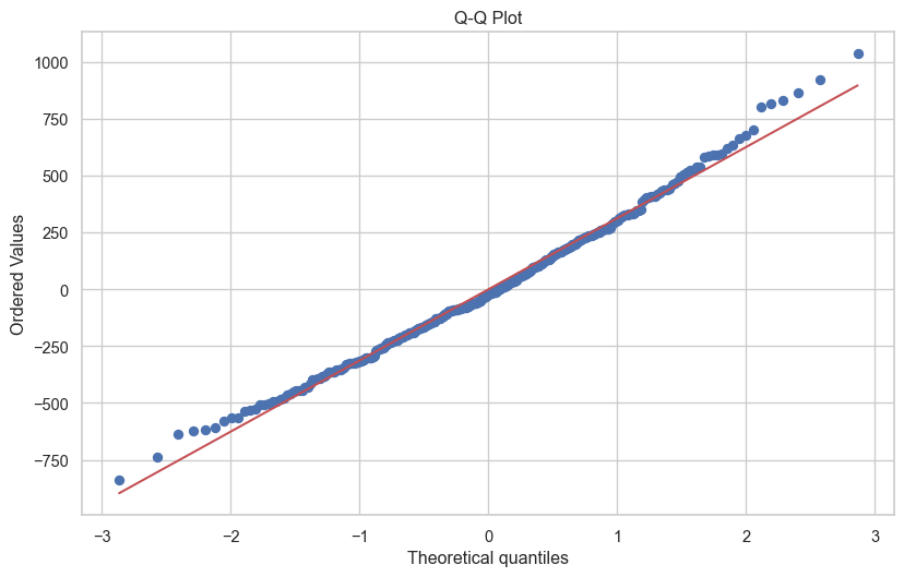

The closer to the red line, the better. However, some deviation is generally fine, and as sample size increases this becomes less of a concern. The very small deviations from the line above are not a cause for concern.

3. Scale-Location Plot (Homoscedasticity)

fig, ax = plt.subplots(figsize=(10, 6))
sns.scatterplot(x=df['fitted'], y=np.sqrt(np.abs(df['standardised_residuals'])), alpha=0.6, ax=ax)
ax.set_xlabel('Fitted Values')
ax.set_ylabel('√|Standardised Residuals|')
ax.set_title('Scale-Location Plot')
plt.show()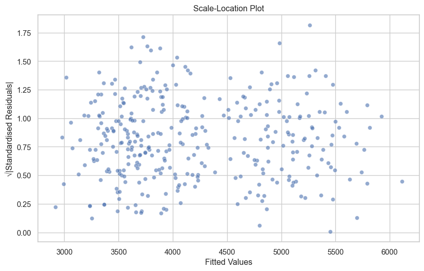

If there is an observable trend or pattern in your Scale-Location plot, this indicates heteroscedasticity.

4. Residuals vs Leverage (Influential Points)

from statsmodels.stats.outliers_influence import OLSInfluence

influence = OLSInfluence(model)
leverage = influence.hat_matrix_diag
cooks_d = influence.cooks_distance[0]

fig, ax = plt.subplots(figsize=(10, 6))
sns.scatterplot(x=leverage, y=df['standardised_residuals'], alpha=0.6, ax=ax)
ax.axhline(y=0, color='red', linestyle='--', linewidth=1)
ax.set_xlabel('Leverage')
ax.set_ylabel('Standardised Residuals')
ax.set_title('Residuals vs Leverage')

# highlight high influence points
high_influence = cooks_d > 4/len(df)
if high_influence.any():
    ax.scatter(leverage[high_influence], df['standardised_residuals'][high_influence], 
               color='red', s=100, alpha=0.6, label='High influence')
    ax.legend()
plt.show()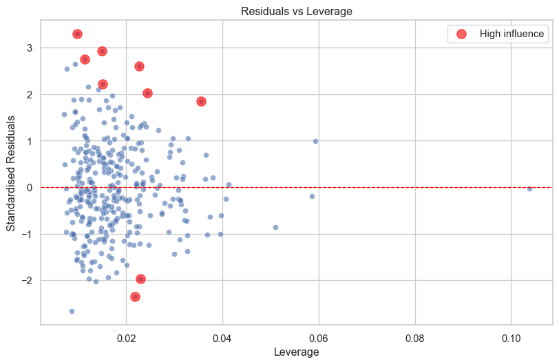

Points that are significantly higher or lower than zero and with high leverage are potentially a problem.

However, I would caution against just removing outliers because they have a significant influence. If those outliers are real observations, should they really be discarded?

Quick Diagnostic Function (Click to Expand)

Let’s create a helper function to generate all diagnostic plots at once.

def plot_diagnostics(model, data=None):
    """
    Create a 2x2 grid of diagnostic plots for a statsmodels regression model.
    
    Parameters:
    -----------
    model : statsmodels regression model
        A fitted statsmodels OLS model
    data : pandas DataFrame, optional
        The data used to fit the model (for some plot enhancements)
    """
    # get residuals and fitted values
    fitted = model.fittedvalues
    residuals = model.resid
    standardised_residuals = model.resid_pearson
    
    # calculate leverage and influence
    influence = OLSInfluence(model)
    leverage = influence.hat_matrix_diag
    
    # create 2x2 plot
    fig, axes = plt.subplots(2, 2, figsize=(14, 10))
    
    # 1. residuals vs fitted
    sns.scatterplot(x=fitted, y=residuals, alpha=0.6, ax=axes[0, 0])
    axes[0, 0].axhline(y=0, color='red', linestyle='--', linewidth=2)
    axes[0, 0].set_xlabel('Fitted Values')
    axes[0, 0].set_ylabel('Residuals')
    axes[0, 0].set_title('Residuals vs Fitted')
    
    # 2. q-q plot
    stats.probplot(residuals, dist="norm", plot=axes[0, 1])
    axes[0, 1].set_title('Q-Q Plot')
    
    # 3. scale-location
    sns.scatterplot(x=fitted, y=np.sqrt(np.abs(standardised_residuals)), alpha=0.6, ax=axes[1, 0])
    axes[1, 0].set_xlabel('Fitted Values')
    axes[1, 0].set_ylabel('√|Standardised Residuals|')
    axes[1, 0].set_title('Scale-Location')
    
    # 4. residuals vs leverage
    sns.scatterplot(x=leverage, y=standardised_residuals, alpha=0.6, ax=axes[1, 1])
    axes[1, 1].axhline(y=0, color='red', linestyle='--', linewidth=1)
    axes[1, 1].set_xlabel('Leverage')
    axes[1, 1].set_ylabel('Standardised Residuals')
    axes[1, 1].set_title('Residuals vs Leverage')
    
    plt.tight_layout()
    plt.show()

# use the function
plot_diagnostics(model_species_sm)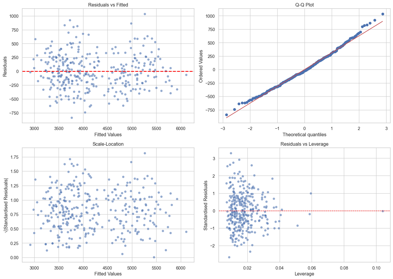

Checking for Multicollinearity

When predictors are highly correlated with each other, coefficient estimates become unstable. We can check this using Variance Inflation Factors (VIF).

from statsmodels.stats.outliers_influence import variance_inflation_factor

# calculate VIF for each predictor
# need to add constant for VIF calculation
X_with_const = sm.add_constant(df[['flipper_len', 'bill_len', 'bill_dep']])

vif_data = pd.DataFrame()
vif_data['Variable'] = X_with_const.columns
vif_data['VIF'] = [variance_inflation_factor(X_with_const.values, i) 
                   for i in range(X_with_const.shape[1])]

print("Variance Inflation Factors:")
print(vif_data)

Variance Inflation Factors:
      Variable         VIF
0        const  691.005294
1  flipper_len    2.633327
2     bill_len    1.850958
3     bill_dep    1.593411

The rule of thumb:

VIF of greater than five = No multicollinearity
VIF of between five and ten = Moderate multicollinearity
VIF greater than ten = High multicollinearity

What Happens When Assumptions Are Violated?

Understanding assumptions helps you know when you can bend or break the rules.

Linearity - Coefficients are biased. Try transformations (log, polynomial) or non-linear models.
Independence - Standard errors are wrong (usually too small). Use clustered standard errors or multilevel models.
Homoscedasticity - Standard errors are wrong. Use robust standard errors (HC3, HC4). Predictions are still unbiased.
Normality - With large samples, not a big problem due to central limit theorem. With small samples, confidence intervals may be wrong.
Multicollinearity - Coefficients are unstable and hard to interpret, but predictions are fine. Remove or combine correlated predictors.

As you gain experience, you’ll learn when violations matter and when they don’t. For now, check diagnostics and flag any concerns.

Summary

sklearn for prediction - Fast, consistent API for building models.
statsmodels for inference - Detailed statistical output for understanding.
Assumptions matter - Check diagnostics, understand when violations are problematic.
Effect sizes over p-values - Focus on what matters practically.

Linear regression is a powerful tool, and learning the principles of linear regression (thinking about predictions, uncertainty, assumptions, and interpretation) apply to much more complex models.

Footnotes

For explanatory models, it is generally best-practice to transform the data so that the intercept is meaningful. For example, subtracting the mean flipper length from each observation (otherwise known as centering) so that the zero value represents the average flipper length and the intercept represents the average body mass for the average flipper length.↩︎
Statistical inference is the process of drawing conclusions about a population (or an effect occurring in the real-world) based on sample data.↩︎
A model with \(\text{R}^2\) = 0.3 can still be incredibly useful if the effects are meaningful and the predictions are good enough for your purpose.↩︎
Fixing the problem can take many shapes. It could involve transforming the data to fit the model better, adding (or removing) variables that improve model fit, or fitting a different type of regression model entirely.↩︎